Data Cleaning in Excel 101, Part 3: How to Combine Columns in Excel

Having the right data in the right columns to meet specific requirements for your analysis plays a major role in the data cleaning process. In Parts 2, 3, and 4 of our Data Cleaning in Excel series, well show you how to solve common issues by utilizing both standard and Excels powerful Flash Fill shortcut.

Part 2 focuses on splitting data from one cell to multiple cells. Here, in Part 3, well cover the opposite: combining data from multiple columns into one column. Coming up in Part 4, well showcase some incredibly useful and time-saving tricks with the mystical powers of Excels Flash Fill function.

Combining Data from Multiple Columns

In our last blog post, we went over how to break apart data that has been exported into just one cell. What about if you have the opposite issue: data in multiple cells that you need to join together? For example, your system may export your donor’s names into first and last names, but you need to put them together in one cell for your next project. How can you put together the data from both cells, and apply the change to an entire column? Try these:

Method #1: CONCATENATE

The Excel formula =CONCATENATE allows you to join together text strings from multiple cells into just one. You can use the formula to combine numbers, text, and characters in addition to cell references.

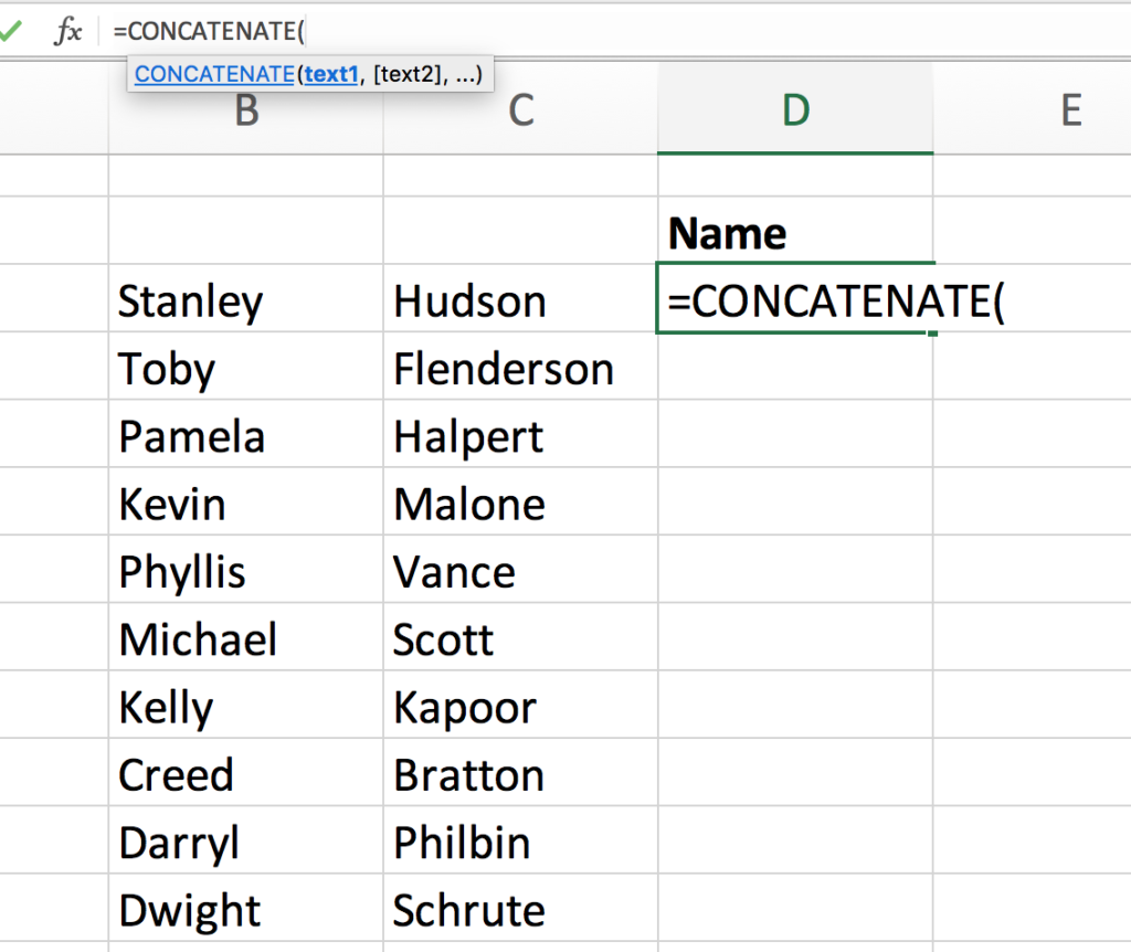
1. Select the cell for your new value, adjacent to your cells you need to combine.
2. Type =CONCATENATE(

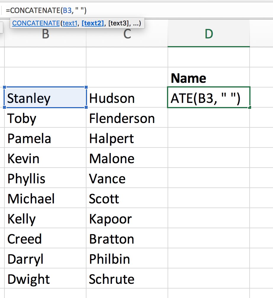
3. Select your first cell reference (first name).

4. Add a **comma **to indicate a new text string.
5. Type to indicate a space between your values.
6. Add another comma.
7. Select your second cell reference (last name).
8. Add a ) to close your parentheses and finish the formula.

9. Click Enter. Your new values will appear.

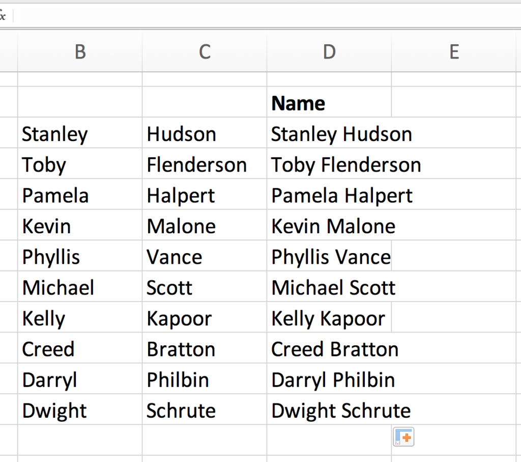
10. **Drag **your formula to fill your new column.

Tip: When simply joining two cells, use an ampersand instead.

No formula required.

Instead of writing the formula, you can use “&” directly between the cells you want to join.

=A1&B1

It’s a shorthand variation of the the =CONCATENATE formula best used when you just need to add two cells. Things get a little more complicated when you need to add a delimiter, or need to use Excel’s formula builder function.

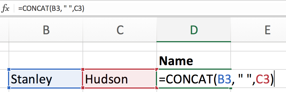
Method #2: CONCAT

Newer versions of Excel (after Excel 2010) have upgraded the =CONCATENATE formula to =CONCAT. The =CONCATENATE formula is still available in every version of Excel to remain compatible with older versions. The difference between the formulas is that =CONCAT can combine cell references in an entire range to fit one cell.

The instructions for use are essentially the same as the =CONCATENATE formula above in method 1. If you want to perform the same function you can do with =CONCATENATE, just type and execute as you normally would (see below).

CONCAT and Range References

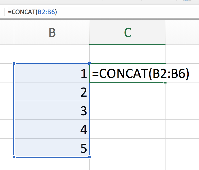
To combine range references, click a cell and expand and drag an entire range.

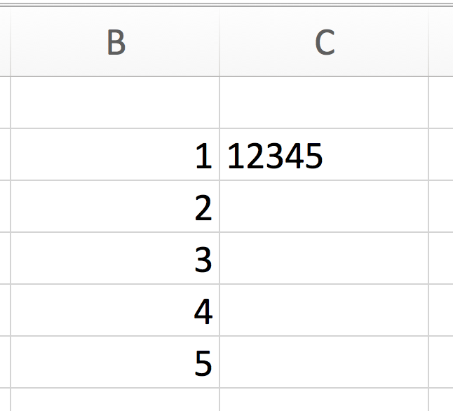
After you execute the formula, your new cell will look like this.

Method 3: TEXTJOIN

If you need to combine a range of cells into text with spaces, commas or another separator, and you dont want to waste time entering it repeatedly between cell references, use =TEXTJOIN. When you type =TEXTJOIN, Excel prompts you to provide: **(delimiter, ignore_empty, text1, [text2], ) **

• delimiter is where you specify what you want to separate the cells. In our case, we would want a , to create spaces between words in our cell references.

-** ignore_empty** is where you choose TRUE or FALSE in regards to including empty cells. If you do want empty cells to be included, type TRUE. Your choice will depend on the data you have and your purposes for combining the text.

• text 1 is the cell reference(s) you must include in your formula to execute the function (including ranges and arrays).
• [text 2] is an optional argument where you can provide additional cell references to combine if you need to.

When filled out, you formula should look like this:

Press Enter, and youll find that TEXTJOIN has combined all of your cell references easily, without having to tediously write between each cell.

Method #4: Flash Fill

Check out our last data cleaning blog post in this series for a review of the Excel function, Flash Fill.

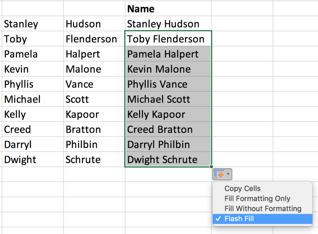
To combine data into one column, well type how we want our new data to look in the cell adjacent to our existing data. Remember, we have to create two entries so Excel can recognize our pattern, and fill in the rest for us.

Stay tuned for Part 4 of our Data Cleaning in Excel series for an in-depth look at the versatility of Flash Fill and some example formats that are sure to inspire you to use the function in your day-to-day work in Excel.

We hope these methods help you as you clean your data! Please let us know if there are other topics or data cleaning problems you would like us to tackle by emailing contact@inciter.io

‍